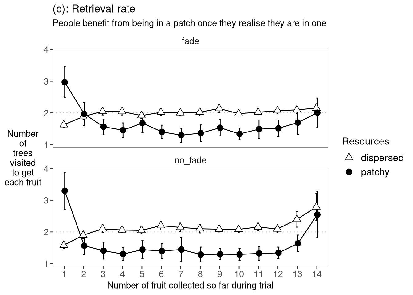
This rate is how many trees they had to look at to get each successive fruit.
e2 Retrieval: Prepare the data
Read the data in and pre-process it.
Show the code
e2 <-readRDS("002-00-e2-data.RDS")# remove things from the raw data to make it # suitable for this particular analysis# remove samples that did not look at a treee2 <- e2 %>%filter(fl>0)# remove the second (and any subsequent) *consecutive* duplicatese2 <- e2 %>%group_by(pp, rr, tb) %>%filter(is.na(tl !=lag(tl)) | tl !=lag(tl)) %>%ungroup()# remove trials where they failed to get 14 fruite2 <- e2 %>%group_by(pp, rr, tb) %>%mutate(max_fr =max(fr)) %>%ungroup() %>%filter(max_fr==14) %>%select(-c(ex, max_fr, st, xx, yy, ln)) # how many trees to get each fruit?# this is neat and it needs to be done after # reducing the data to row-per-valid-tree-visite2$ntrees_to_get_a_fruit =NAj =0for (k inseq_along(e2$ix)) { j = j +1if (e2[k, 'fl']==2) { e2[k, 'ntrees_to_get_a_fruit'] = j j =0 }}# remove any remaining NAse2 <- e2 %>%filter(!is.na(ntrees_to_get_a_fruit))# average over trials (and ignore stage) to yield # participant means suitable for ggplot and ANOVArtv = e2 %>%select(ff, pp, rr, tb, fr, ntrees_to_get_a_fruit) %>%group_by(ff, pp, rr, fr) %>%summarise(mu=mean(ntrees_to_get_a_fruit)) %>%ungroup() %>%mutate(ff=as_factor(ff), pp=as_factor(pp), rr=as_factor(rr), fr=as_factor(fr))saveRDS(rtv, "e2_retrieval_plot_data.rds")
The effect of fading was F(1, 40) = 0.36, p=0.554.
The effect of resources was F(1, 40) = 71.71, p<.001.
The effect of fruit was F(5.3, 211.7) = 17.22, p<.001.
The fruit x resources interaction was F(6.1, 244.2) = 32.17, p<.001.
The fruit x fading interaction was F(5.3, 211.7) = 2.89, p<.05.
The fruit x fading interaction was F(5.3, 211.7) = 2.89, p<.05.
e2 Retrieval: Plot
Ten points along the x axis, each participant contributes one point per cell, facet on fading
Show the code
ggplot(data=rtv, aes(x=fr, y=mu, group=rr, fill=rr, shape=rr)) +facet_wrap(~ff, nrow=2)+labs(title="(c): Retrieval rate", subtitle="People benefit from being in a patch once they realise they are in one")+ylab("Number\nof\ntrees\nvisited\nto get\neach fruit")+xlab("Number of fruit collected so far during trial")+ my_fgms_theme+geom_hline(yintercept=2, lty=3,col="grey")+scale_fill_manual(name="Resources", values=c("white", "black")) +scale_shape_manual(name="Resources", values=c(24,19)) +stat_summary(fun.data = mean_cl_normal, geom ="errorbar", width=0.2, position=pd) +stat_summary(fun = mean, geom ="line", position=pd) +stat_summary(fun = mean, geom ="point", size=3, position=pd)