Trees

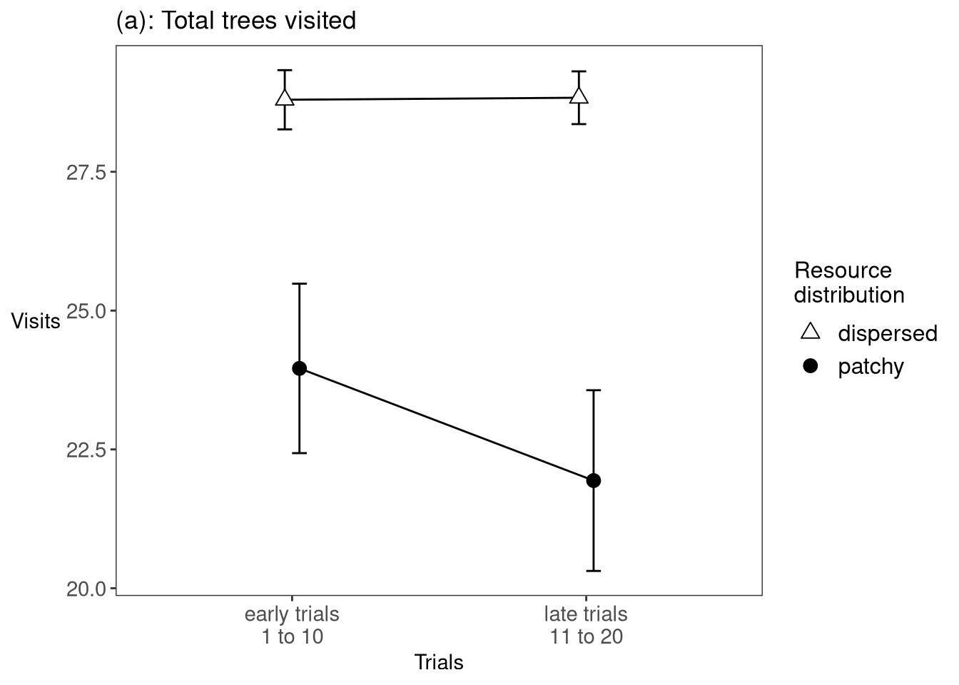
This number is how many trees they looked at overall to get the fourteen out of fifteen fruit - high numbers represent worse performance.

E2 Ntrees: Prepare the data

Read the data in and pre-process it.

Show the code

e2 <- readRDS("002-00-e2-data.RDS")

# remove things from the raw data to make it 
# suitable for this particular analysis

# remove samples that did not look at a tree
e2 <- e2 %>% filter(fl>0)

# remove the second (and any subsequent) *consecutive* duplicates
e2 <- e2 %>% 
  group_by(ff, pp, rr, tb) %>% 
  filter(is.na(tl != lag(tl)) | tl != lag(tl)) %>% 
  ungroup()

# remove trials where they failed to get 14 fruit
e2 <- e2 %>% 
  group_by(ff, pp, rr, tb) %>% 
  mutate(max_fr = max(fr)) %>% 
  ungroup() %>% 
  filter(max_fr==14)

# average over tree-visits to get counts for each trial
ntr.counts <- e2 %>% 
  select(ff, pp, rr, st, tb, tl) %>% 
  group_by(ff, pp, rr, st, tb) %>% 
  summarise(ntrees=n()) %>% 
  ungroup() %>% 
  mutate(ff=as_factor(ff), pp=as_factor(pp), rr=as_factor(rr),  st=as_factor(st))

# average over trials to get mean count for each stage
ntr <- ntr.counts %>% 
  group_by(ff, pp, rr, st) %>% 
  summarise(mean_ntrees_per_stage=mean(ntrees)) %>% 
  ungroup()

saveRDS(ntr, "e2_ntrees_plot_data.rds")

E2 Ntrees: ANOVA

Run the ANOVA

Show the code

options(contrasts=c("contr.sum","contr.poly"))
e2_ntrees_ANOVA <- 
  ezANOVA(data=ntr,
          dv=mean_ntrees_per_stage,
          wid=pp,
          within=c(rr, st),
          between=ff,
          type=3,
          return_aov = TRUE)

Warning: Data is unbalanced (unequal N per group). Make sure you specified a
well-considered value for the type argument to ezANOVA().

Show the code

if("Sphericity Corrections" %in% names(e2_ntrees_ANOVA)){
  corr=aovSphericityAdjustment(e2_ntrees_ANOVA)$ANOVA %>% tibble()
} else {
  corr=e2_ntrees_ANOVA$ANOVA %>% tibble()  
  }

Do we care about unbalanced anova? There were 22 subjects in fade but 20 in no_fade.

Table the ANOVA.

Show the code

prettify_anova(e2_ntrees_ANOVA, "e2 Ntrees ANOVA")

e2 Ntrees ANOVA
Effect	DFn	DFd	F	p	sig
ff	1	40	0.37	0.545
rr	1	40	71.44	0.000	***
st	1	40	22.33	0.000	***
ff:rr	1	40	2.88	0.097
ff:st	1	40	8.92	0.005	**
rr:st	1	40	28.22	0.000	***
ff:rr:st	1	40	6.32	0.016	*

Report the anova

Main effects

The effect of fading was F(1, 40) = 0.37, p=0.545.

The effect of resources was F(1, 40) = 71.44, p<.001.

The effect of stage was F(1, 40) = 22.33, p<.001.

Two-way interactions

The effect of fading x stage was F(1, 40) = 8.92, p<.01.

The effect of resources x stage was F(1, 40) = 28.22, p<.001.

plots

Show the code

ggplot(data=ntr, aes(x=st, y=mean_ntrees_per_stage, group=rr, fill=rr, shape=rr)) + 
  #facet_wrap(~ff) +
  ggtitle("(a): Total trees visited")+
  ylab("Visits")+
  xlab("Trials")+
  my_fgms_theme+  
  scale_fill_manual(name="Resource\ndistribution",values=c("white", "black")) +
  scale_shape_manual(name="Resource\ndistribution",values=c(24,19)) +
  stat_summary(fun.data = mean_cl_normal, geom = "errorbar", width=0.1, position=pd) +
  stat_summary(fun = mean, geom = "line", position=pd) + 
  stat_summary(fun = mean, geom = "point", size=3, position=pd)+
  scale_x_discrete(labels=c("early trials\n1 to 10", "late trials\n11 to 20"))

Means

Table means for resources

Show the code

rrpremeans = ntr %>% group_by(rr, pp, st) %>%
  summarise(mu=mean(mean_ntrees_per_stage)) %>% 
  summarise(mu=mean(mu)) 
rrmeans <- rrpremeans %>% 
  summarise(mean=mean(mu), sd=sd(mu))
prettify_means(rrmeans, "E2 Number of trees resources means")

E2 Number of trees resources means
rr	mean	sd
dispersed	28.82	1.51
patchy	22.95	4.89

Table means for stage

Show the code

frpremeans = ntr %>% group_by(st, pp, rr) %>%
  summarise(mu=mean(mean_ntrees_per_stage)) %>% 
  summarise(mu=mean(mu))  
frmeans <- frpremeans %>% 
  summarise(mean=mean(mu), sd=sd(mu))
prettify_means(frmeans, "E2 Number of trees stage means")

E2 Number of trees stage means
st	mean	sd
early	26.38	2.84
late	25.39	2.91