Chapter 5 Retrieval Rate

Experiment 1

e1 <- readRDS("001-00-e1-data.RDS")

# remove things from the raw data to make it suitable for this particular analysis

# remove samples that did not look at a tree
e1 <- e1 %>% filter(fl>0)

# remove the second (and any subsequent) *consecutive* duplicates
e1 <- e1 %>% 
  group_by(pp, rr, tb) %>% 
  filter(is.na(tl != lag(tl)) | tl != lag(tl)) %>% 
  ungroup()

# remove trials where they failed to get 10 fruit
e1 <- e1 %>% 
  group_by(pp, te) %>% 
  mutate(max_fr = max(fr)) %>% 
  ungroup() %>% 
  filter(max_fr==10)

# how many trees to get each fruit?
# this is neat and it needs to be done after reducing the data to row-per-valid-tree-visit
e1$ntrees_to_get_a_fruit = NA
j = 0
for (k in seq_along(e1$ix)) {
 j = j + 1
 if (e1[k, 'fl']==2) {
   e1[k, 'ntrees_to_get_a_fruit'] = j
   j = 0
 }
}

# remove any remaining NAs
e1 <- e1 %>% filter(!is.na(ntrees_to_get_a_fruit))

# average over trials (and ignore stage) to yield participant means suitable for ggplot and ANOVA
rtv = e1 %>% 
  select(pp, rr, tb, fr, ntrees_to_get_a_fruit) %>% 
  group_by(pp, rr, fr) %>% 
  summarise(mu=mean(ntrees_to_get_a_fruit)) %>% 
  ungroup() %>% 
  mutate(pp=as_factor(pp), rr=as_factor(rr), fr=as_factor(fr))

saveRDS(rtv, "e1_retrieval_plot_data.rds")

5.1 ANOVA

options(contrasts=c("contr.sum","contr.poly"))
e1_retrievalrate_ANOVA <- 
  ezANOVA(data=rtv,
          dv=mu,
          wid=pp,
          within=c(rr, fr),
          type=3, return_aov = TRUE)

prettify_anova(e1_retrievalrate_ANOVA, "Retrieval rate")

Table 5.1: Retrieval rate
Effect	DFn	DFd	F	sig
rr	1	41	54.14	***
fr	9	369	22.99	***
rr:fr	9	369	46.85	***

prettify_anova(aovSphericityAdjustment(e1_retrievalrate_ANOVA), "Retrieval rate")

Table 5.1: Retrieval rate
Effect	DFn	DFd	F	sig
rr	1.0	41.0	54.14	***
fr	3.9	160.4	22.99	***
rr:fr	4.8	197.9	46.85	***

The effect of fruit (\(F(9, 369) = 22.99\), \(p < .001\), \(\hat{\eta}^2_G = .204\), 90% CI \([.133, .250]\))

The effect of fruit after Greenhouse-Geisser correction for sphericity violation was F(3.91, 160.43) = 22.99, p< .001

The fruit x resources interaction after Greenhouse-Geisser correction for sphericity violation was F(4.83, 197.91) = 46.85, p< .001

5.2 Plot

# Ten points along the x axis, each participant contributes one point per cell

ggplot(
  data=rtv, 
  aes(x=fr, y=mu, group=rr, pch=rr, fill=rr)
) +
  theme_bw()+
  theme(aspect.ratio = 1, panel.grid=element_blank())+
  scale_fill_manual(name="Resources", values=c("white", "black")) +
  scale_shape_manual(name="Resources", values=c(24,19)) +
  stat_summary(fun.data = mean_cl_normal, geom = "errorbar", width=0.2, position=position_dodge(0.25)) +
  stat_summary(fun = mean, geom = "line", position=position_dodge(0.25)) + 
  stat_summary(fun = mean, geom = "point", size=3, position=position_dodge(0.25))+
  ylab("Mean number of trees visited to get each fruit")+
  xlab("Fruit index")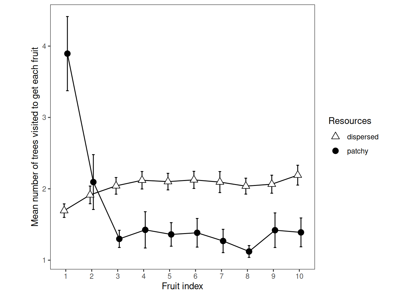

5.3 Resources Means

rrpremeans = rtv %>% group_by(rr, pp, fr) %>%
  summarise(mu=mean(mu)) %>% 
  summarise(mu=mean(mu)) 
rrmeans <- rrpremeans %>% 
  summarise(mean=mean(mu), sd=sd(mu))
prettify_means(rrmeans, "stage means")

Table 5.2: stage means
rr	mean	sd
dispersed	2.04	0.13
patchy	1.67	0.30

5.4 Fruit means

frpremeans = rtv %>% group_by(fr, pp, rr) %>%
  summarise(mu=mean(mu)) %>% 
  summarise(mu=mean(mu))  
frmeans <- frpremeans %>% 
  summarise(mean=mean(mu), sd=sd(mu))
prettify_means(frmeans, "fruit means")

Table 5.3: fruit means
fr	mean	sd
1	2.79	0.90
2	2.00	0.63
3	1.67	0.28
4	1.77	0.44
5	1.73	0.36
6	1.75	0.38
7	1.68	0.35
8	1.58	0.20
9	1.74	0.44
10	1.79	0.38